


This article discusses four bottlenecks in modern data stack applications and introduces a number of tools, some of which are new, for identifying and removing them. These bottlenecks could occur in any framework but a particular emphasis will be given to Apache Spark and PySpark.
The applications/riddles discussed below have something in common: They require around 10 minutes wall clock time when a “local version” of them is run on a commodity notebook. Using more or more powerful processors or machines for their execution would not significantly reduce their run time. But there are also important differences: Each riddle contains a different kind of bottleneck that is responsible for the slowness and each of these bottlenecks will be identified with a different approach. Some of these analytical tools are innovative or not widely used, references to source code are included in the second part of this article. The first section will discuss the riddles in a “black box” manner:
The Fatso
The fatso occurs frequently in the modern data stack. A symptom of running a local version of it is noise – the fans of my notebook are very active for almost 10 minutes, the entire application lifetime. Since we can rarely listen to machines in a cluster computing environment, we need a different approach to identify a fatso:
JVM Profile
The following code snippet (full version here) combines two information sources, the output of a JVM profiler and normal Spark logs, into a single visualization:
profile_file = './data/ProfileFatso/CpuAndMemoryFatso.json.gz'  # Output from JVM profiler
profile_parser = ProfileParser(profile_file, normalize=True)
data_points: List[Scatter] = profile_parser.make_graph()

logfile = './data/ProfileFatso/JobFatso.log.gz'  # standard Spark logs
log_parser = SparkLogParser(logfile)
stage_interval_markers: Scatter = log_parser.extract_stage_markers()
data_points.append(stage_interval_markers)

layout = log_parser.extract_job_markers(700)
fig = Figure(data=data_points, layout=layout)
plot(fig, filename='fatso.html')
The interactive graph produced by running this script can be analyzed in its full glory here, a smaller snapshot is displayed below:
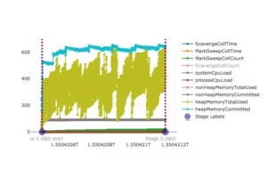
Spark’s execution model consists of different units of different “granularity levels” and some of these are displayed above: Boundaries of Spark jobs are represented as vertical dashed lines, start and end points of Spark stages are displayed as transparent blue dots on the x-axis which also show the full stage names/IDs. This scheduling information does not add a lot of insight here since Fatso consists of only one Spark job which in turn consists of just a single Spark stage (comprised of three tasks) but, as shown below, knowing such time points can be very helpful when analyzing more complex applications.
For all graphs in this article, the x-axis shows the application run time as UNIX Epoch time (milliseconds passed since 1 January 1970). The y-axis represents different normalized units for different metrics: For graph lines representing memory metrics such as total heap memory used (“heapMemoryTotalUsed”, ocher green line above), it represents gigabytes; for time measurements like MarkSweep GC collection time (“MarkSweepCollTime”, orange line above), data points on the y-axis represent milliseconds. More details can be found in this data structure which can be changed or extended with new metrics from different profilers.
One available metric, ScavengeCollCount, is absent from the snapshot above but present in the original. It signifies a minor garbage collection event and almost increases linearly up to 20000 during Fatso’s execution. In other words, the application ran for almost 10 minutes – from epoch 1550420474091 (= 17/02/2019 16:21:14) until epoch 1550421148780 (= 17/02/2019 16:32:28) – and more than 20000 minor Garbage Collection events and almost 70 major GC events (“MarkSweepCollCount”, green line) occurred.
When the application was launched, no configuration parameters were manually set so the default Spark settings applied. This means that the maximum memory available to the program was 1GB. Having a closer look at the two heap memory metrics heapMemoryCommitted and heapMemoryTotalUsed reveals that both lines approach this 1GB ceiling near the end of the application.
The intermediate conclusion that can be drawn from the discussion so far is that the application is very memory hungry and a lot of GC activity is going on, but the exact reason for this is still unclear. A second tool can help now:
JVM FlameGraph
The profiler also collected stacktraces which can be folded and transformed into flame graphs with the help of my fold_stacks.py script and this external script:
Phils-MacBook-Pro:analytics a$ python3 fold_stacks.py ./analytics/data/ProfileFatso/StacktraceFatso.json.gz > Fatso.folded
Phils-MacBook-Pro:analytics a$ perl flamegraph.pl Fatso.folded > FatsoFlame.svg
Opening FatsoFlame.svg in a browser shows the following, the full version which is also searchable (top right corner) is located at this location:

Click for Full Size
A rule of thumb for the interpretation of flame graphs is: The more spiky the shape, the better. We see many plateaus above with native Spark/Java functions like sun.misc.unsafe.park sitting on top (first plateau) or low-level functions from packages like io.netty occurring near the top, this is a 3rd party library that Spark depends on for network communication / IO. The only functions in the picture that are defined by me are located in the center plateau, searching for the package name profile.sparkjob in the top right corner will prove this claim. On top of these user defined functions are native Java Array and String functions; a closer look at the definition of fatFunctionOuter and fatFunctionInner would reveal that they create many String objects in an efficient way so we have identified the two Fatso methods that need to be optimized.
Python/PySpark Profiles
What about Spark applications written in Python? I created several PySpark profilers that try to provide some of the functionality of Uber’s JVM profiler. Because of the architecture of PySpark, it might be beneficial to generate both Python and JVM profiles in order to get a good grasp of the overall resource usage. This can be accomplished for the Python edition of Fatso by using the following launch command (abbreviated, full command here):
~/spark-2.4.0-bin-hadoop2.7/bin/spark-submit \
--conf spark.python.profile=true \
--conf spark.driver.extraJavaOptions=-javaagent:/.../=sampleInterval=1000,metricInterval=100,reporter=...outputDir=... \
./spark_jobs/job_fatso.py cpumemstack /users/phil/phil_stopwatch/analytics/data/profile_fatso > Fatso_PySpark.log
The –conf parameter in the third line is responsible for attaching the JVM profiler. The –conf parameter in the second line as well as the two script arguments in the last line are Python specific and required for PySpark profiling: The cpumemstack argument will choose a PySpark profiler that captures both CPU/memory usage as well as stack traces. By providing a second script argument in the form of a directory path, it is ensured that the profile records are written into separate output files instead of just printing all of them to the standard output.
Similar to its Scala cousin, the PySpark edition of Fatso completes in around 10 minutes on my MacBook and creates several JSON files in the specified output directory. The JVM profile could be visualized idenpendently of the Python profile but it might be more insightful to create a single combined graph from them. This can be accomplished easily and is shown in the second half of this script. The full combined graph is located here
The clever reader will already have a hunch about the high memory consumption and who is responsible for it: The garbage collection activity of the JVM that is again represented by MarkSweepCollCount and ScavengeCollCount is much lower here compared to the “pure” Spark run described in the previous paragraphs (20000 events above versus less than 20 GC events now). The two inefficient fatso functions are now implemented in Python and therefore not managed by the JVM leading to far fewer JVM memory usage and GC events. A PySpark flamegraph should confirm our hunch:
Phils-MacBook-Pro:analytics a$ python3 fold_stacks.py ./analytics/data/profile_fatso/s_8_stack.json  > FatsoPyspark.folded
Phils-MacBook-Pro:analytics a$ perl flamegraph.pl  FatsoPyspark.folded  > FatsoPySparkFlame.svg
Opening FatsoPySparkFlame.svg in a browser displays …

Click for Full Size
And indeed, two fatso methods sit ontop the stack for almost 90% of all measurements burning most CPU cycles. It would be easy to create a combined JVM/Python flamegraph by concatenating the respective stacktrace files. This would be of limited use here though since the JVM flamegraph will likely consist entirely of native Java/Spark functions over which a Python coder has no control. One scenario I can think of where this merging of JVM with PySpark stacktraces might be especially useful is when Java code or libraries are registered and called from PySpark/Python code which is getting easier and easier in newer versions of Spark. In the discussion of Slacker later on, I will present a combined stack trace of Python and Scala code.
The Straggler
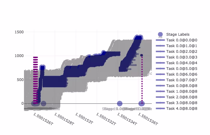
The Straggler is deceiving: It appears as if all resources are fully utilized most the time and only closer analysis can reveal that this might be the case for only a small subset of the system or for a limited period of time. The following graph created from this script combines two CPU metrics with information about task and stage boundaries extracted from the standard logging output of a typical straggler run; the full size graph can be investigated here
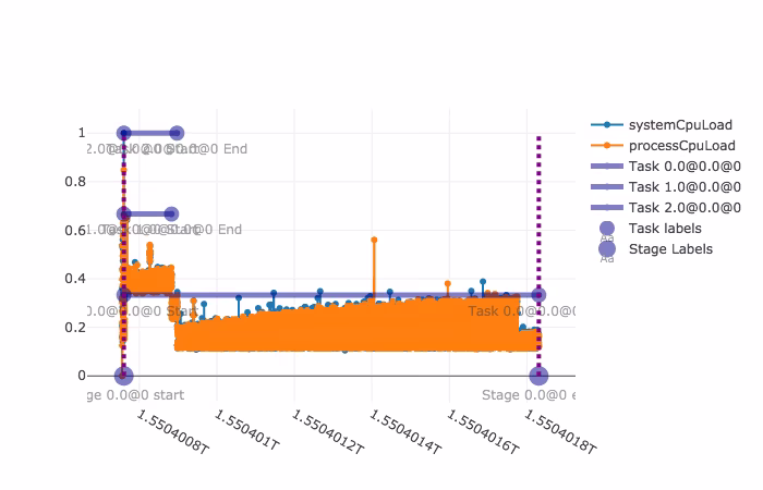
The associated application consisted of one Spark job which is represented as vertical dashed lines at the left and right. This single job was comprised of a single stage, shown as transparent blue dots on the x axis that coincide with the job start and end points. But there were three tasks within that stage so we can see three horizontal task lines. The naming schema of this execution hierarchy is not arbitrary:
- The stage name in the graph is 0.0@0 because a stage with the id 0.0 which belonged to a job with id 0 is referred to. The first part of stage or task names is a floating point number, this reflects the apparent naming convention in Spark logs that new attempts of failed task or stages are baptized with an incremented fraction part.
- The task names are 0.0@0.0@0, 1.0@0.0@0, and 2.0@0.0@0 because three tasks were launched that were all members of stage 0.0@0 that in turn belonged to job 0
The three tasks have the same start time which almost coincides with the application’s invocation but very different end times: Tasks 1.0@0.0@0 and 2.0@0.0@0 finish within the first fifth of the application’s lifetime whereas task 0.0@0.0@0 stays alive for almost the entire application since its start and end points are located at the left and right borders of this graph. The orange and light blue lines visualize two CPU metrics (system cpu load and process cpu load) whose fluctuations correspond with the task activity: We can observe that the CPU load drops right after tasks 1.0@0.0@0 and 2.0@0.0@0 end. It stays at around 20% for 4/5 of the time, when only straggler task 0.0@0.0@0 is running.
Concurrency Profiles
When an application consists of more than just one stage with three tasks like Straggler, it might be more illuminating to calculate and represent the total number of tasks that were running at any point during the application’s lifetime. The “concurrency profile” of a modern data stack workload might look more like

The source code that is the basis for the graph can be found in this script. The big difference to the Straggler toy example before is that in real-life applications, many different log files are compiled (one for each container/Spark executor) and there is only one “master” log file which contains necessary information about scheduling and task boundaries which are needed to make concurrency profiles. The script uses an AppParser class that does this automatically by creating a list of LogParser objects (one for each container) and then parsing them to determine the master log. We can attempt a back-of-the-envelope calculation to increase the efficiency of the application from just looking at this concurrency profile: In case around 80 physical CPU cores were used (given multiple peaks of ~80 active tasks), we can hypothesize that the application was “overallocated” by at least 20 CPU cores or 4 to 7 Spark executors or one to three nodes as Spark executors are often configured to use 3 to 5 physical CPU cores. Reducing the machines reserved for this application should not increase its execution time but it will give more resources to other users in a shared cluster setting or save some $$ in a cloud environment.
A Fratso
What about the specs of the actual compute nodes used? The memory profile for a similar app created via this code segment is chaotic yet illuminating since more than 50 Spark executors/containers were launched by application and each one left its mark in the graph in the form of a memory metric line (original located here)
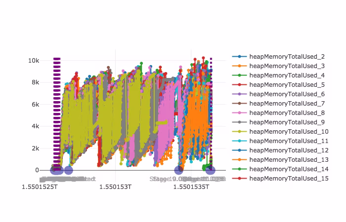
The peak heap memory used is a little more than 10GB, one executor crosses this 10k line twice (top right) while most other executors use at most 8-9 GB or less. Removing the memory usage from the picture and displaying scheduling information like task boundaries instead results in the following graph
The application launches several small Spark jobs initially as indicated by the occurrence of multiple dashed lines near the left border. However, more than 90% of the total execution time is consumed by a single big job which has the ID 8. A closer look at the blue dots on the x-axis that represent boundaries of Spark stages reveals that there are two longer stages within job 8. During the first stage, there are four task waves without stragglers – concurrent tasks that together look like solid blue rectangles when visualized this way. The second stage of job 8 does have a straggler task as there is one horizontal blue task line that is much longer active than its “neighbour” tasks. Looking back at the memory graph of this application, it is likely that this straggler task is also responsible for the heap memory peak of >10GB that we discovered. We might have identified a “fratso” here (a straggling fatso) and this task/stage should definitely be analyzed in more detail when improving the associated application.
The script that generated all three previous plots can be found here.
The Heckler: CoreNLP & spaCy
Applying NLP or machine learning methods often involves the use of third party libraries which in turn create quite memory-intensive objects. There are several different ways of constructing such heavy classifiers in Spark so that each task can access them, the first version of the Heckler code that is the topic of this section will do that in the worst possible way. I am not aware of a metric currently exposed by Spark that could directly show such inefficiencies, something similar to a measure of network transfer from master to executors would be required for one case below. The identification of this bottleneck must therefore happen indirectly by applying some more sophisticated string matching and collapsing logic to Spark’s standard logs:
log_file = './data/ProfileHeckler1/JobHeckler1.log.gz'
log_parser = SparkLogParser(log_file)
collapsed_ranked_log: List[Tuple[int, List[str]]] = log_parser.get_top_log_chunks()
for line in collapsed_ranked_log[:5]:  # print 5 most frequently occurring log chunks
    print(line)
Executing the script containing this code segment produces the following output:
Phils-MacBook-Pro:analytics a$ python3 extract_heckler.py

^^ Identified time format for log file: %Y-%m-%d %H:%M:%S

(329, ['StanfordCoreNLP:88 - Adding annotator tokenize', 'StanfordCoreNLP:88 - Adding annotator ssplit',
'StanfordCoreNLP:88 - Adding annotator pos', 'StanfordCoreNLP:88 - Adding annotator lemma',
'StanfordCoreNLP:88 - Adding annotator parse'])
(257, ['StanfordCoreNLP:88 - Adding annotator tokenize', 'StanfordCoreNLP:88 - Adding annotator ssplit',
'StanfordCoreNLP:88 - Adding annotator pos', 'StanfordCoreNLP:88 - Adding annotator lemma',
'StanfordCoreNLP:88 - Adding annotator parse'])
(223, ['StanfordCoreNLP:88 - Adding annotator tokenize', 'StanfordCoreNLP:88 - Adding annotator ssplit',
'StanfordCoreNLP:88 - Adding annotator pos', 'StanfordCoreNLP:88 - Adding annotator lemma',
'StanfordCoreNLP:88 - Adding annotator parse'])
(221, ['StanfordCoreNLP:88 - Adding annotator tokenize', 'StanfordCoreNLP:88 - Adding annotator ssplit',
'StanfordCoreNLP:88 - Adding annotator pos', 'StanfordCoreNLP:88 - Adding annotator lemma',
'StanfordCoreNLP:88 - Adding annotator parse'])
(197, ['StanfordCoreNLP:88 - Adding annotator tokenize', 'StanfordCoreNLP:88 - Adding annotator ssplit',
'StanfordCoreNLP:88 - Adding annotator pos', 'StanfordCoreNLP:88 - Adding annotator lemma',
'StanfordCoreNLP:88 - Adding annotator parse'])
These are the 5 most frequent log chunks found in the logging file, each one is a pair [int, List[str]]. The left integer signifies the total number of times the right list of log segments occurred in the file; each individual member in the list occurred in a separate log line in the file. Hence the return value of the method get_top_log_chunks that created the output above has the type annotation List[Tuple[int, List[str]]], it extracts a ranked list of contiguous log segments.
The top record can be interpreted the following way: The four strings
StanfordCoreNLP:88 - Adding annotator tokenize
StanfordCoreNLP:88 - Adding annotator ssplit
StanfordCoreNLP:88 - Adding annotator pos
StanfordCoreNLP:88 - Adding annotator lemma
StanfordCoreNLP:88 - Adding annotator parse
occurred as infixes in this order 329 times in total in the log file. They were likely part of longer log lines as normalization and collapsing logic was applied by the extraction algorithm, an example occurrence of the first part of the chunk (StanfordCoreNLP:88 – Adding annotator tokenize) would be
2019-02-16 08:44:30 INFO StanfordCoreNLP:88 - Adding annotator tokenizeWhat does this tell us? The associated Spark app seems to have performed some NLP tagging since log4j messages from the Stanford CoreNLP project can be found as part of the Spark logs. Initializing a StanfordCoreNLP object …
  val props = new Properties()
  props.setProperty("annotators", "tokenize,ssplit,pos,lemma,parse")

  val pipeline = new StanfordCoreNLP(props)
  val annotation = new Annotation("This is an example sentence")

  pipeline.annotate(annotation)
  val parseTree = annotation.get(classOf[SentencesAnnotation]).get(0).get(classOf[TreeAnnotation])
  println(parseTree.toString) // prints (ROOT (NP (NN Example) (NN sentence)))
0 [main] INFO edu.stanford.nlp.pipeline.StanfordCoreNLP  - Adding annotator tokenize
9 [main] INFO edu.stanford.nlp.pipeline.StanfordCoreNLP  - Adding annotator ssplit
13 [main] INFO edu.stanford.nlp.pipeline.StanfordCoreNLP  - Adding annotator pos
847 [main] INFO edu.stanford.nlp.tagger.maxent.MaxentTagger  - Loading POS tagger from [...] done [0.8 sec].
848 [main] INFO edu.stanford.nlp.pipeline.StanfordCoreNLP  - Adding annotator lemma
849 [main] INFO edu.stanford.nlp.pipeline.StanfordCoreNLP  - Adding annotator parse
1257 [main] INFO edu.stanford.nlp.parser.common.ParserGrammar  - Loading parser from serialized [...] ... done [0.4 sec].
… which tells us that five annotators (tokenize, ssplit, pos, lemma, parse) are created and wrapped inside a single StanfordCoreNLP object. Concerning the use of CoreNLP with Spark, the number of cores/tasks used in Heckler is three (as it is in all other riddles) which means that we should find at most three occurrences of these annotator messages in the corresponding Spark log file. But we already saw more than 1000 occurrences when only the top 5 log chunks were investigated above. Having a closer look at the Heckler source code resolves this contradiction, the implementation is bad since one classifier object is recreated for every input sentence that will be syntactially annotated – there are 60000 input sentences in total so an StanfordCoreNLP object will be constructed a staggering 60000 times. Due to the distributed/concurrent nature of Heckler, we don’t always see the annotator messages in the order tokenize – ssplit – pos – lemma – parse because log messages of task (1) might interweave with log messages of task (2) and (3) in the actual log file which is also the reason for the slightly reordered log chunks in the top 5 list.
Improving this inefficient implementation is not too difficult: Creating the classifier inside a mapPartitions instead of a map function as done here will only create three StanfordCoreNLP objects overall. However, this is not the minimum, I will now set the record for creating the smallest number of tagger objects with the minimum amount of network transfer: Since StanfordCoreNLP is not serializable per se, it needs to be wrapped inside a class that is in order to prevent a java.io.NotSerializableException when broadcasting it later:
class DistribbutedStanfordCoreNLP extends Serializable {
  val props = new Properties()
  props.setProperty("annotators", "tokenize,ssplit,pos,lemma,parse")
  lazy val pipeline = new StanfordCoreNLP(props)
}
[...]
val pipelineWrapper = new DistribbutedStanfordCoreNLP()
val pipelineBroadcast: Broadcast[DistribbutedStanfordCoreNLP] = session.sparkContext.broadcast(pipelineWrapper)
[...]
val parsedStrings3 = stringsDS.map(string => {
   val annotation = new Annotation(string)
   pipelineBroadcast.value.pipeline.annotate(annotation)
   val parseTree = annotation.get(classOf[SentencesAnnotation]).get(0).get(classOf[TreeAnnotation])
   parseTree.toString
})
The proof lies in the logs:
19/02/23 18:48:45 INFO Executor: Running task 1.0 in stage 0.0 (TID 1)
19/02/23 18:48:45 INFO Executor: Running task 0.0 in stage 0.0 (TID 0)
19/02/23 18:48:45 INFO Executor: Running task 2.0 in stage 0.0 (TID 2)
19/02/23 18:48:46 INFO StanfordCoreNLP: Adding annotator tokenize
19/02/23 18:48:46 INFO StanfordCoreNLP: Adding annotator ssplit
19/02/23 18:48:46 INFO StanfordCoreNLP: Adding annotator pos
19/02/23 18:48:46 INFO MaxentTagger: Loading POS tagger from [...] ... done [0.6 sec].
19/02/23 18:48:46 INFO StanfordCoreNLP: Adding annotator lemma
19/02/23 18:48:46 INFO StanfordCoreNLP: Adding annotator parse
19/02/23 18:48:47 INFO ParserGrammar: Loading parser from serialized file edu/stanford/nlp/models/lexparser/englishPCFG.ser.gz ... done [0.4 sec].
19/02/23 18:59:07 INFO Executor: Finished task 0.0 in stage 0.0 (TID 0). 1590 bytes result sent to driver
19/02/23 18:59:07 INFO Executor: Finished task 2.0 in stage 0.0 (TID 2). 1590 bytes result sent to driver
19/02/23 18:59:07 INFO Executor: Finished task 1.0 in stage 0.0 (TID 1). 1590 bytes result sent to driver
I’m not sure about the multi-threading capabilities of StanfordCoreNLP so it might turn out that the second “per partition” solution is superior performance-wise to the third. In any case, we reduced the number of tagging objects created from 60000 to three or one, not bad.
spaCy on PySpark
The PySpark version of Heckler will use spaCy (written in Cython/Python) as NLP library instead of CoreNLP. From the perspective of a JVM aficionado, packaging in Python itself is odd and spaCy doesn’t seem to be very chatty. Therefore I created an initialization function that should print more log messages and address potential issues when running spaCy in a distributed environment as its model files need to be present on every Spark executor.
As expected, the “bad” implementation of Heckler recreates one spaCy NLP model per input sentence as proven by this logging excerpt:
[Stage 0:>                                                          3 / 3]
^^ Using spaCy 2.0.18
^^ Model found at /usr/local/lib/python3.6/site-packages/spacy/data/en_core_web_sm
^^ Using spaCy 2.0.18
^^ Model found at /usr/local/lib/python3.6/site-packages/spacy/data/en_core_web_sm
^^ Using spaCy 2.0.18
^^ Model found at /usr/local/lib/python3.6/site-packages/spacy/data/en_core_web_sm
^^ Created model en_core_web_sm
^^ Created model en_core_web_sm
^^ Created model en_core_web_sm
^^ Using spaCy 2.0.18
^^ Model found at /usr/local/lib/python3.6/site-packages/spacy/data/en_core_web_sm
^^ Using spaCy 2.0.18
^^ Model found at /usr/local/lib/python3.6/site-packages/spacy/data/en_core_web_sm
^^ Using spaCy 2.0.18
^^ Model found at /usr/local/lib/python3.6/site-packages/spacy/data/en_core_web_sm
^^ Created model en_core_web_sm
^^ Created model en_core_web_sm
^^ Created model en_core_web_sm
[...]
Inspired by the Scala edition of Heckler, the “per partition” PySpark solution only initialize three spacy NLP objects during the application’s lifetime, the complete log file of that run is short:
[Stage 0:>                                                          (0 + 3) / 3]
^^ Using spaCy 2.0.18
^^ Using spaCy 2.0.18
^^ Using spaCy 2.0.18
^^ Model found at /usr/local/lib/python3.6/site-packages/spacy/data/en_core_web_sm
^^ Model found at /usr/local/lib/python3.6/site-packages/spacy/data/en_core_web_sm
^^ Model found at /usr/local/lib/python3.6/site-packages/spacy/data/en_core_web_sm
^^ Created model en_core_web_sm
^^ Created model en_core_web_sm
^^ Created model en_core_web_sm
1500
Finding failure messages
The functionality introduced in the previous paragraphs can be modified to facilitate the investigation of failed applications: The reason for a crash is often not immediately apparent and requires sifting through log files. Resource-intensive applications will create numerous log files (one per container/Spark executor) so search functionality along with deduplication and pattern matching logic should come in handy here: The function extract_errors from the AppParser class tries to deduplicate potential exceptions and error messages and will print them out in reverse chronological order. An exception or error message might occur several times during a run with slight variations (e.g., different timestamps or code line numbers) but the last occurrence is the most important one for debugging purposes since it might be the direct cause for the failure.
app_path = './data/application_1549675138635_0005'
app_parser = AppParser(app_path)
app_errors: Deque[Tuple[str, List[str]]] = app_parser.extract_errors()

for error in app_errors:
    print(error)
^^ Identified app path with log files
^^ Identified time format for log file: %y/%m/%d %H:%M:%S
^^ Warning: Not all tasks completed successfully: {(16.0, 9.0, 8), (16.1, 9.0, 8), (164.0, 9.0, 8), ...}
^^ Extracting task intervals
^^ Extracting stage intervals
^^ Extracting job intervals

Error messages found, most recent ones first:

(‘/users/phil/data/application_1549_0005/container_1549_0001_02_000002/stderr.gz’, [‘18/02/01 21:49:35 ERROR ApplicationMaster: User class threw exception: org.apache.spark.SparkException: Job aborted.’, ‘org.apache.spark.SparkException: Job aborted.’, ‘at org.apache.spark.sql.execution.datasources.FileFormatWriteranonfun$write$1.apply(FileFormatWriter.scala:166)’, ‘at org.apache.spark.sql.execution.SQLExecution$.withNewExecutionId(SQLExecution.scala:65)’, ‘at org.apache.spark.sql.execution.datasources.FileFormatWriter$.write(FileFormatWriter.scala:166)’, ‘at org.apache.spark.sql.execution.datasources.InsertIntoHadoopFsRelationCommand.run(InsertIntoHadoopFsRelationCommand.scala:145)’, ‘at org.apache.spark.sql.execution.command.ExecutedCommandExec.sideEffectResult$lzycompute(commands.scala:58)’, ‘at org.apache.spark.sql.execution.command.ExecutedCommandExec.sideEffectResult(commands.scala:56)’, ‘at org.apache.spark.sql.execution.command.ExecutedCommandExec.doExecute(commands.scala:74)’, ‘at org.apache.spark.sql.execution.SparkPlananonfun$executeQuery$1.apply(SparkPlan.scala:138)’, ‘at org.apache.spark.rdd.RDDOperationScope$.withScope(RDDOperationScope.scala:151)’, ‘at org.apache.spark.sql.execution.SparkPlan.executeQuery(SparkPlan.scala:135)’, ‘at org.apache.spark.sql.execution.SparkPlan.execute(SparkPlan.scala:116)’, ‘at org.apache.spark.sql.execution.QueryExecution.toRdd$lzycompute(QueryExecution.scala:92)’, ‘at org.apache.spark.sql.execution.QueryExecution.toRdd(QueryExecution.scala:92)’, ‘at org.apache.spark.sql.execution.datasources.DataSource.writeInFileFormat(DataSource.scala:435)’, ‘at org.apache.spark.sql.execution.datasources.DataSource.write(DataSource.scala:471)’, ‘at org.apache.spark.sql.execution.datasources.SaveIntoDataSourceCommand.run(SaveIntoDataSourceCommand.scala:50)’, ‘at org.apache.spark.sql.execution.command.ExecutedCommandExec.sideEffectResult$lzycompute(commands.scala:58)’, ‘at org.apache.spark.sql.execution.command.ExecutedCommandExec.sideEffectResult(commands.scala:56)’, ‘at org.apache.spark.sql.execution.command.ExecutedCommandExec.doExecute(commands.scala:74)’, ‘at org.apache.spark.sql.execution.SparkPlananonfun$executeQuery$1.apply(SparkPlan.scala:138)’, ‘at org.apache.spark.rdd.RDDOperationScope$.withScope(RDDOperationScope.scala:151)’, ‘at org.apache.spark.sql.execution.SparkPlan.executeQuery(SparkPlan.scala:135)’, ‘at org.apache.spark.sql.execution.SparkPlan.execute(SparkPlan.scala:116)’, ‘at org.apache.spark.sql.execution.QueryExecution.toRdd$lzycompute(QueryExecution.scala:92)’, ‘at org.apache.spark.sql.execution.QueryExecution.toRdd(QueryExecution.scala:92)’, ‘at org.apache.spark.sql.DataFrameWriter.runCommand(DataFrameWriter.scala:609)’, ‘at org.apache.spark.sql.DataFrameWriter.save(DataFrameWriter.scala:233)’, ‘at org.apache.spark.sql.DataFrameWriter.save(DataFrameWriter.scala:217)’, ‘at org.apache.spark.sql.DataFrameWriter.parquet(DataFrameWriter.scala:508)’, […] ‘… 48 more’])

(‘/users/phil/data/application_1549_0005/container_1549_0001_02_000124/stderr.gz’, [‘18/02/01 21:49:34 ERROR CoarseGrainedExecutorBackend: RECEIVED SIGNAL TERM’])

(‘/users/phil/data/application_1549_0005/container_1549_0001_02_000002/stderr.gz’, [‘18/02/01 21:49:34 WARN YarnAllocator: Container marked as failed: container_1549731000_0001_02_000124 on host: ip-172-18-39-28.ec2.internal. Exit status: -100. Diagnostics: Container released on a lost node’])

(‘/users/phil/data/application_1549_0005/container_1549_0001_02_000002/stderr.gz’, [‘18/02/01 21:49:34 WARN YarnSchedulerBackend$YarnSchedulerEndpoint: Container marked as failed: container_1549731000_0001_02_000124 on host: ip-172-18-39-28.ec2.internal. Exit status: -100. Diagnostics: Container released on a lost node’])

(‘/users/phil/data/application_1549_0005/container_1549_0001_02_000002/stderr.gz’, [‘18/02/01 21:49:34 ERROR TaskSetManager: Task 30 in stage 9.0 failed 4 times; aborting job’])

(‘/users/phil/data/application_1549_0005/container_1549_0001_02_000002/stderr.gz’, [‘18/02/01 21:49:34 ERROR YarnClusterScheduler: Lost executor 62 on ip-172-18-39-28.ec2.internal: Container marked as failed: container_1549731000_0001_02_000124 on host: ip-172-18-39-28.ec2.internal. Exit status: -100. Diagnostics: Container released on a lost node’])

(‘/users/phil/data/application_1549_0005/container_1549_0001_02_000002/stderr.gz’, [‘18/02/01 21:49:34 WARN TaskSetManager: Lost task 4.3 in stage 9.0 (TID 610, ip-172-18-39-28.ec2.internal, executor 62): ExecutorLostFailure (executor 62 exited caused by one of the running tasks) Reason: Container marked as failed: container_1549731000_0001_02_000124 on host: ip-172-18-39-28.ec2.internal. Exit status: -100. Diagnostics: Container released on a lost node’])

(‘/users/phil/data/application_1549_0005/container_1549_0001_02_000002/stderr.gz’, [‘18/02/01 21:49:34 WARN ExecutorAllocationManager: No stages are running, but numRunningTasks != 0’])

[…]
Each error record printed out in this fashion consists of two elements: The first one is a path to the source log to the source log in which the second element, the actual error chunk, was found. The error chunk is a single or multiline error message to which collapsing logic was applied and is stored in a list of strings. The application that threw the errors shown above seems to have crashed because some problems occurred during a write phase since classes like FileFormatWriter occur in the final stack trace that was produced by executor container_1549_0001_02_000002. It is likely that not enough output partitions were used when materializing output records to a storage layer. The total number of error chunks in all container log files associated with this application was more than 350, the deduplication logic of AppParser.extract_errors boiled this high number down to less than 20.
The Slacker
The Slacker does exactly what the name suggests – not a lot. Let’s collect and investigate the maximum values of its most important metrics:
combined_file = './data/profile_slacker/CombinedCpuAndMemory.json.gz'  # Output from JVM & PySpark profilers

jvm_parser = ProfileParser(combined_file)
jvm_parser.manually_set_profiler('JVMProfiler')

pyspark_parser = ProfileParser(combined_file)
pyspark_parser.manually_set_profiler('pyspark')

jvm_maxima: Dict[str, float] = jvm_parser.get_maxima()
pyspark_maxima: Dict[str, float] = pyspark_parser.get_maxima()

print('JVM max values:')
print(jvm_maxima)
print('\nPySpark max values:')
print(pyspark_maxima)
The output is …
JVM max values:
{'ScavengeCollTime': 0.0013, 'MarkSweepCollTime': 0.00255, 'MarkSweepCollCount': 3.0, 'ScavengeCollCount': 10.0,
'systemCpuLoad': 0.64, 'processCpuLoad': 0.6189945167759597, 'nonHeapMemoryTotalUsed': 89.079,
'nonHeapMemoryCommitted': 90.3125, 'heapMemoryTotalUsed': 336.95, 'heapMemoryCommitted': 452.0}
PySpark max values:
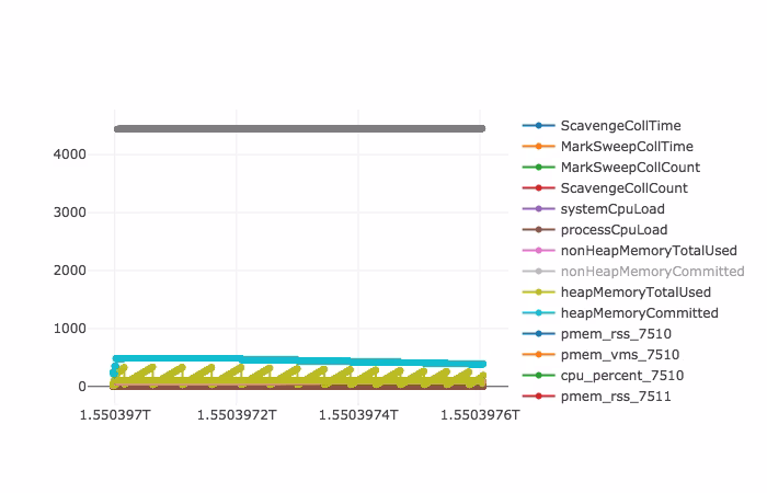
{'pmem_rss': 78.50390625, 'pmem_vms': 4448.35546875, 'cpu_percent': 0.4}These are low values given a baseline overhead of running Spark and especially when comparing them to the profiles for Fatso above – for example, only 13 GC events happened and the peak CPU load for the entire run was less than 65%. Visualizing all CPU data points shows that these maxima occurred at the beginning / end of the application when there is always lots of initialization and cleanup work going on regardless of the actual code being executed (bigger version here):

So the system is almost idle for the majority of the time. The slacker in this pure form is a rare sight; when processing real-life workloads, slacking most likely occurs in certain stages that interact with an external system like querying a database for records that should be joined with Datasets/RDDs later on or that materialize output records to a storage layer like HDFS and use not enough write partitions. A combined flame graph of JVM and Python stack traces will reveal the slacking part:

Click for Full Size
In the first plateau which is also the longest, two custom Python functions sit at the top. After inspecting their implementation here and there, the low system utilization should not be surprising anymore: The second function from the top,job_slacker.py:slacking, is basically a simple loop that calls a function helper.py:secondsSleep from an external helper package many times. This function has a sample presence of almost 20% (seen in the original) and, since it sits atop the plateau, is executed by the CPU most of the time. As its function name suggests, it causes the program to sleep for one second. So Slacker is essentially a 10 minute long system sleep. In real-world modern data stack applications that have slacking phases, we can expect the top of many plateaus to be occupied by “write” functions like FileFormatWriter$$anonfun$write$1.apply(FileFormatWriter.scala or by functions related to DB queries.
Source Code & Links & Goodies
Quite a lot of things were discussed and code exists that implements every idea presented:
Riddle source code
The Spark source code for the riddles is located in this repository:
The PysSpark editions along with all log and profile parsing logic can be found in the main repo:
Profiling the JVM
Uber’s recently open sourced JVM profiler isn’t the first of its kind but has a number of features that are very handy for the cases described in this article: It is “non-invasive” so source code doesn’t need to be changed at all in order to collect metrics. Any JVM can be profiled which means that this project is suitable for tracking a Spark master as well as its associated executors. Internally this profiler uses the java.lang.management interface that was introduced with Java 1.5 and accesses several Bean objects.
When running the riddles mentioned above in local mode, only one JVM is launched and the master subsumes the executors so only a –conf spark.driver.extraJavaOptions= has to be added to the launch command, a distributed application also requires a second –conf spark.executor.extraJavaOptions=. Full launch commands are included in my project’s repo
Phil’s PysSpark profilers
I implemented three custom PySpark profilers here which should provide functionality similar to that of Uber’s JVM profiler for a PySpark user: A CPU/memory profiler, a stack profiler for creating PySpark flamegraphs and a combination of the two. Detais about how to integrate them into an application can be found in the project’s readme file.
Going distributed
If the JVM profiler is used as described above, three different types of records are generated which, in case the FileOutputReporter flag is used, are written to three separate JSON files, ProcessInfo.json, CpuAndMemory.json, and Stacktrace.json. The ProcessInfo.json file contains meta information and is not used in this article. Similarly, my PySpark profilers will create one or two different types of output records that are stored in at least two JSON files with the pattern s_X_stack.json or s_X_cpumem.json_ when sparkContext.dump_profiles(dump_path). If sparkContext.show_profiles() is used instead, all profile records would be written to the standard output.
In a distributed/cloud environment, Uber’s and my FileOutputReporter might not be able to create output files on storage systems like HDFS or S3 so the profiler records might need to be written to the standard output files (stdout.gz) instead. Since the design of the profile and application parsers in parsers.py is compositional, this is not a problem. A demonstration of how to extract both metrics and scheduling info from all standard output files belonging to an application is here.
When launching a distributed application, Spark executors run on multiple nodes in a cluster and produce several log files, one per executor/container. In a cloud environment like AWS, these log files will be organized in the following structure:
s3://aws-logs/elasticmapreduce/clusterid-1/containers/application_1_0001/container_1_001/
                                                                                         stderr.gz
                                                                                         stdout.gz
s3://aws-logs/elasticmapreduce/clusterid-1/containers/application_1_0001/container_1_002/
                                                                                         stderr.gz
                                                                                         stdout.gz
[...]
s3://aws-logs/elasticmapreduce/clusterid-1/containers/application_1_0001/container_1_N/
                                                                                         stderr.gz
                                                                                         stdout.gz

[...]

s3://aws-logs/elasticmapreduce/clusterid-M/containers/application_K_0001/container_K_L/
                                                                                         stderr.gz
                                                                                         stdout.gz
An EMR cluster like clusterid-1 might run several Spark applications consecutively, each one as its own step. Each application launched a number of containers, application_1_0001 for example launched executors container_1_001, container_1_002, …, container_1_N. Each of these container created a standard error and a standard out file on S3. In order to analyze a particular application like application_1_0001 above, all of its associated log files like …/application_1_0001/container_1_001/stderr.gz and …/application_1_0001/container_1_001/stdout.gz are needed. The easiest way is to collect all files under the application folder using a command like …
aws s3 cp --recursive s3://aws-logs/elasticmapreduce/clusterid-1/containers/application_1_0001/ ./application_1_0001/
… and then to create an AppParser object like
from parsers import AppParser
app_path = './application_1_0001/'  # path to the application directory downloaded from s3 above
app_parser = AppParser(app_path)
This object creates a number of SparkLogParser objects internally (one for each container) and automatically identifies the “master” log file created by the Spark driver (likely located under application_1_0001/container_1_001/). Several useful functions are now made available by the app_parser object, examples can be found in this script and more detailed explanations are in the readme file.