Table of Contents
In this blog post, I’ll set up and run a couple of experiments to demonstrate the effects of different kinds of partition pruning in Spark.
Big data has a complex relationship with SQL, which has long served as the standard query language for traditional databases – Oracle, Microsoft SQL Server, IBM DB2, and a vast number of others.
Only relational databases support true SQL natively, and many big data databases fall in the NoSQL – ie, non-relational – camp. For these databases, there are a number of near-SQL alternatives.
When dealing with big data, the most crucial part of processing and answering any SQL or near-SQL query is likely to be the I/O cost – that is, moving data around, including making one or more copies of the same data, as the query processor gathers needed data and completes the response to the query.
A great deal of effort has gone into reducing I/O costs for queries. Some of the techniques used are indexes, columnar data storage, data skipping, etc.
Partition pruning, described below, is one of the data skipping techniques used by most of the query engines like Spark, Impala, and Presto. One of the advanced ways of partition pruning is called dynamic partition pruning. In this blog post, we will work to understand both of these concepts and how they impact query execution, while reducing I/O requirements.
What is Partition Pruning?
Let’s first understand what partition pruning is, how it works, and the implications of this for performance.
If a table is partitioned and one of the query predicates is on the table partition column(s), then only partitions that contain data which satisfy the predicate get scanned. Partition pruning eliminates scanning of the partitions which are not required by the query.
There are two types of partition pruning.
- Static partition pruning. Partition filters are determined at query analysis/optimize time.
- Dynamic partition pruning. Partition filters are determined at runtime, looking at the actual values returned by some of the predicates.
Experiment Setup
For this experiment we have created three Hive tables, to mimic real-life workloads on a smaller scale. Although the number of tables is small, and their data size almost insignificant, the findings are valuable to clearly understand the impact of partition pruning, and to gain insight into some of its intricacies.
Spark version used : 3.0.1
Important configuration settings for our experiment :
- spark.sql.cbo.enabled = false (default)
- spark.sql.cbo.joinReorder.enabled = false (default)
- spark.sql.adaptive.enabled = false (default)
- spark.sql.optimizer.dynamicPartitionPruning.enabled = false (default is true)
We have disabled dynamic partition pruning for the first half of the experiment to see the effect of static partition pruning.
| Table Name | Columns | Partition column | Row Count | Num Partitions |
| T1 | key, val | key | 21,000,000 | 1000 |
| T2 | dim_key, val | dim_key | 800 | 400 |
| T3 | key, val | key | 11,000,000 | 1000 |
Static Partition Pruning
We will begin with the benefits of static partition pruning, and how they affect table scans.
Let’s first try with a simple join query between T1 & T2.
| select t1.key from t1,t2 where t1.key=t2.dim_key |
Query Plan
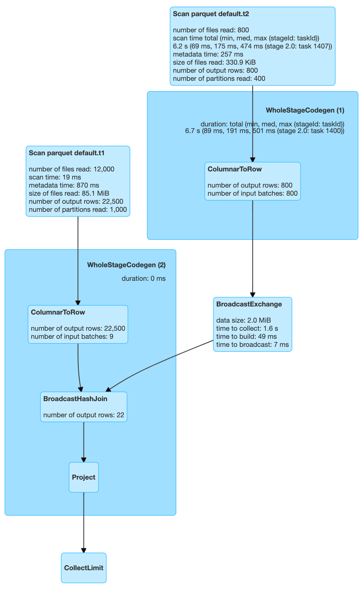
This query scans all 1000 partitions of T1 and all 400 partitions of T2. So in this case no partitions were pruned.
Let’s try putting a predicate on T1’s partition column.
| select t1.key from t1 ,t2 where t1.key=t2.dim_key and t1.key = 40 |
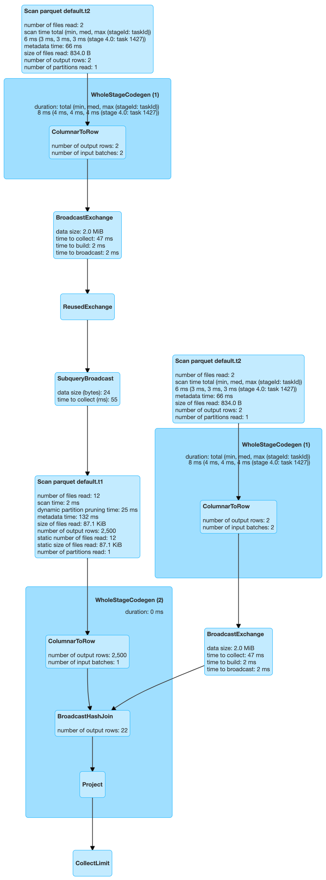
What happened here? As we added the predicate “t1.key = 40,” and “key” is a partitioning column, that means the query requires data from only one partition, which is reflected in the “number of partitions read” on the scan operator for T1.
But there is another interesting thing. If you observe the scan operator for T2, it also says only one partition is read. Why?
If we deduce logically, we need:
- All rows from T1 where t1.key = 40
- All rows from T2 where t2.dim_key = t1.key
- Hence, all rows from T2 where t2.dim_key = 40
- All rows of T2 where t2.dim_key=40 can be only be in one partition of T2, as it’s a partitioning column
What if the predicate would have been on T2, rather than T1? The end result would be the same. You can check yourself.
| select t1.key from t1,t2 where t1.key=t2.dim_key and t2.dim_key = 40 |
What if the predicate satisfies more than one partition? The ultimate effect would be the same. The query processor would eliminate all the partitions which don’t satisfy the predicate.
| select t1.key from t1 ,t2 where t1.key=t2.dim_key and t2.dim_key > 40 and t2.dim_key < 100 |
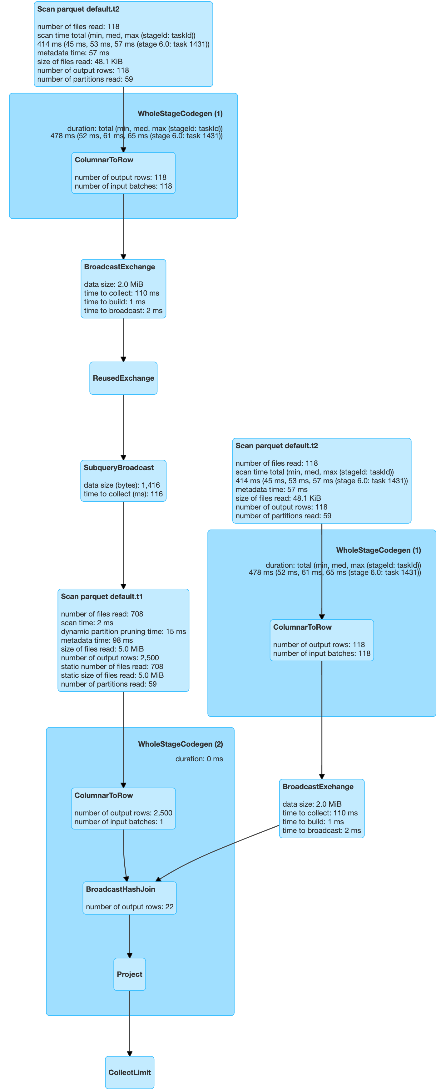 As we can see, there are 59 partitions which are scanned from each table. Still a significant saving as compared to scanning 1000 partitions.
So far, so good. Now let’s try adding another table, T3, to the mix.
| select t1.key from t1, t3, t2 where t1.key=t3.key and t1.val=t3.val and t1.key=t2.dim_key and t2.dim_key = 40 |
Something strange happened here. As expected, only one partition was scanned for both T1 and T2. But 1000 partitions were scanned for T3.
This is a bit odd. If we extend our logic above, only one partition should have been picked up for T3 as well. It was not so.
Let’s try the same query, arranged a bit differently. Here we have just changed the order of join tables. The rest of the query is the same.
| select t1.key from t1, t2, t3 where t1.key=t3.key and t1.val=t3.val and t1.key=t2.dim_key and t2.dim_key = 40 |
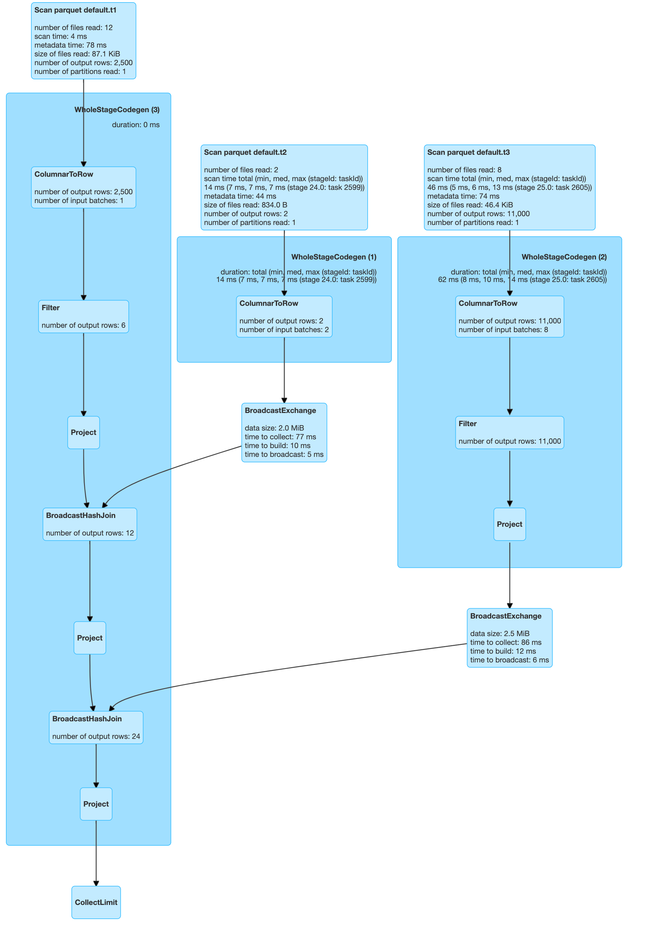
Now we can see the query scanned one partition from each of the tables. So is the join order important for static partition pruning? It should not be, but we see that it is. This looks like it’s a limitation in Spark 3.0.1.
Dynamic Partition Pruning
So far, we have looked at queries which have one predicate on a partitioning column(s) of tables – key, dim_key etc. What will happen if the predicate is on a non-partitioned column of T2, like “val”?
Let’s try such a query.
| select t1.key from t1, t2 where t1.key=t2.dim_key and t2.val > 40 |
As you might have guessed, all the partitions of both the tables are scanned. Can we optimize this, given that the size of T2 is very small ? Can we eliminate certain partitions from T1, knowing the fact that predicates on T2 may select data from only a subset of its partitions?
This is where dynamic partition pruning will help us. Let’s re-enable it.
| set spark.sql.optimizer.dynamicPartitionPruning.enabled=true
|
Then, re-run the above query.
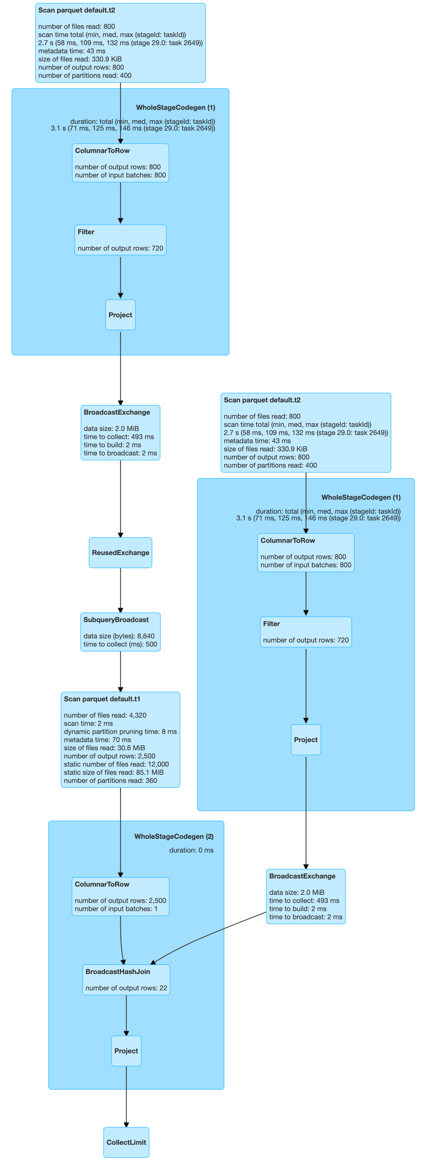
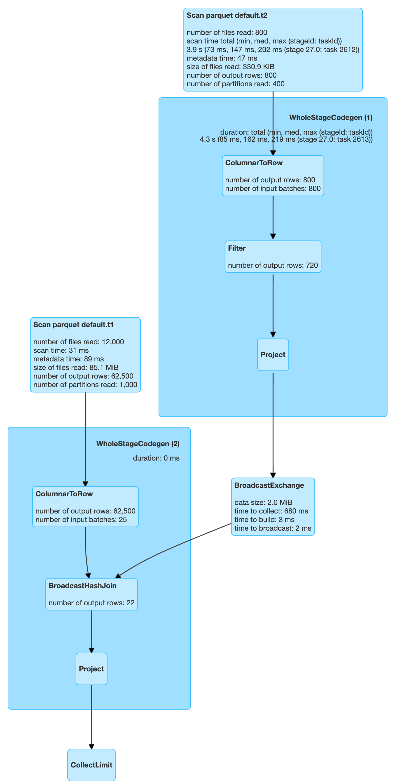
As we can see, although all 400 partitions were scanned for T2, only 360 partitions were scanned for T1. We won’t go through the details of dynamic partition pruning (DPP). A lot of materials already exist on the web, such as the following:
Dynamic Partition Pruning in Apache Spark Bogdan Ghit Databricks -Juliusz Sompolski (Databricks).
You can read about how DPP is implemented in the above blogs. Our focus is its impact on the queries.
Now that we have executed a simple case, let’s fire off a query that’s a bit more complex.
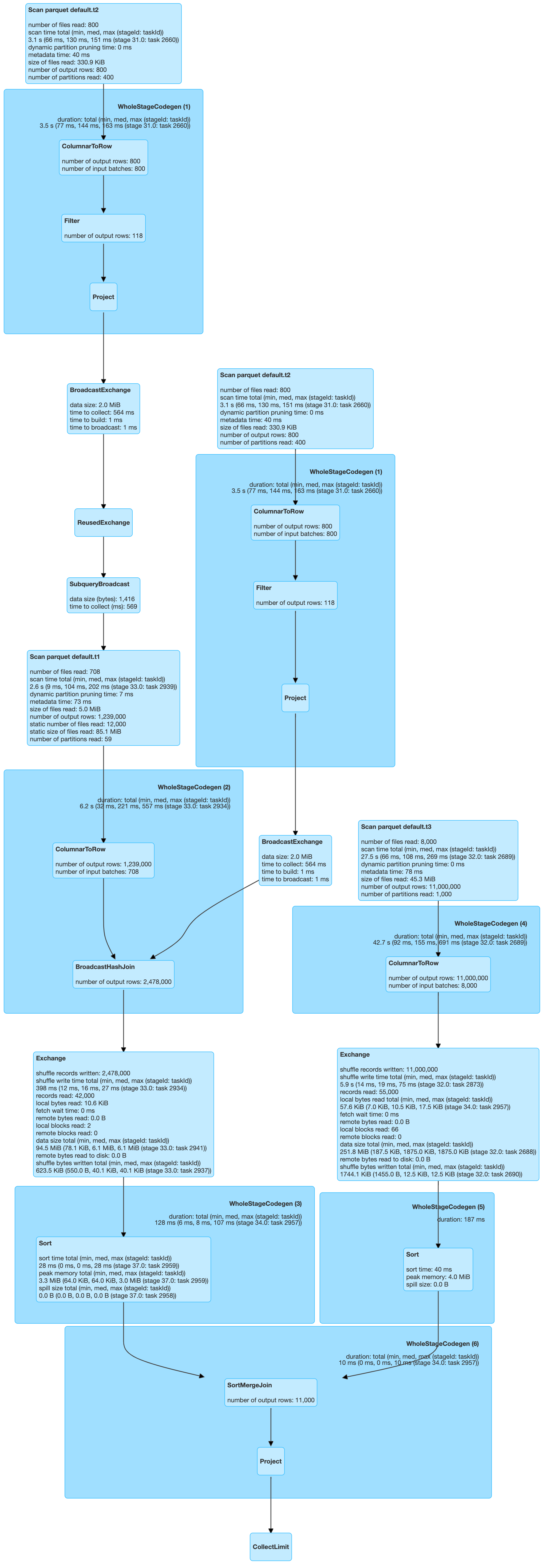
| select t1.key from t1, t2, t3 where t1.key=t3.key and t3.key=t2.dim_key and t1.key=t2.dim_key and t2.val > 40 and t2.val < 100 |

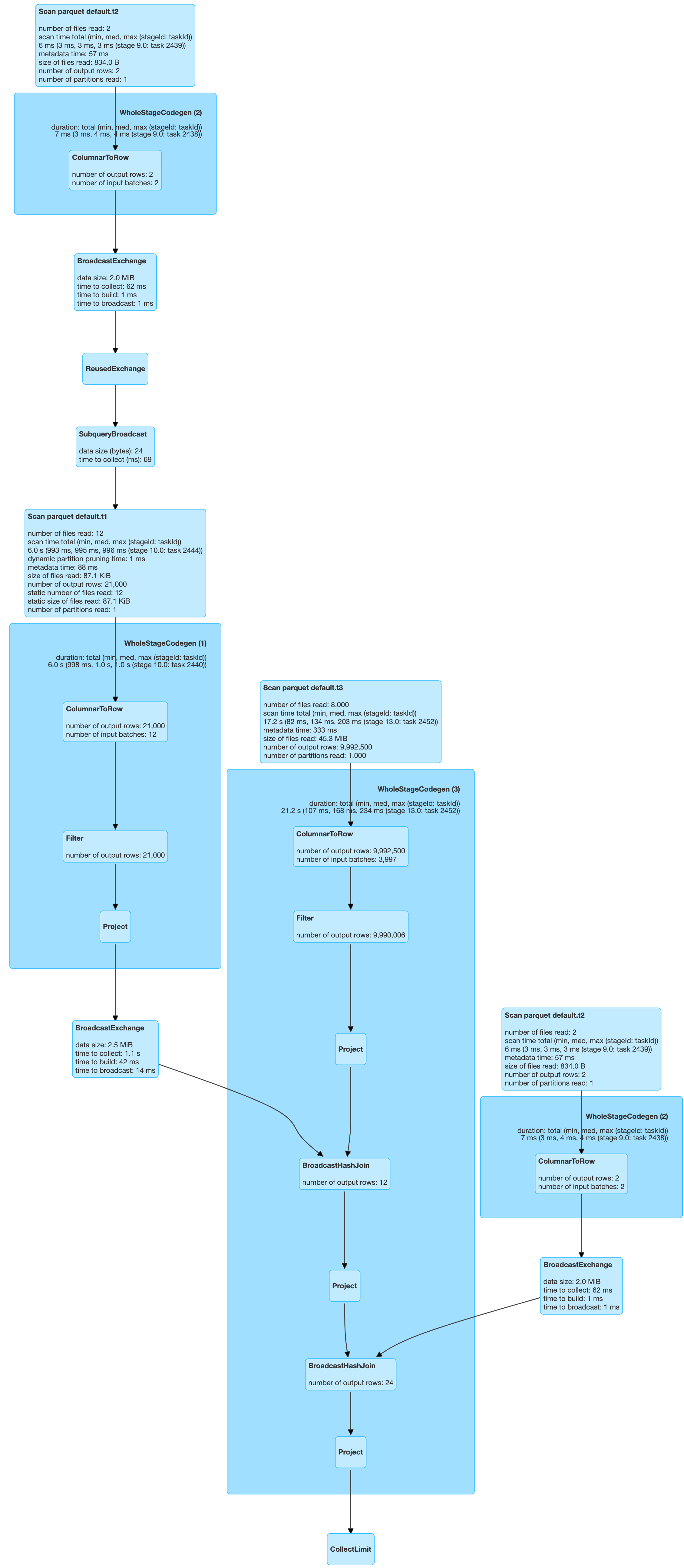
A lot of interesting things are going on here. As before, scans of T1 got the benefit of partition pruning. Only 59 partitions of T1 got scanned. But what happened to T3? All 1000 partitions were scanned.
To investigate the problem, I checked Spark’s code. I found that, at the moment, only a single DPP subquery is supported in Spark.
Ok, but how does this affect query writers? Now it becomes more important to get our join order right so that a more costly table can get help from DPP. For example, if the above query were written as shown below, with the order of T1 and T3 changed, what would be the impact?
| select t1.key from t3, t2, t1 where t1.key=t3.key and t3.key=t2.dim_key and t1.key=t2.dim_key and t2.val > 40 and t2.val < 100 |
You guessed it! DPP will be applied to T3 rather than T1, which will not be very helpful for us, as T1 is almost twice the size of T3.
That means in certain cases join order is very important. Isn’t it the job of the optimizer, more specifically the “cost-based optimizer” (CBO), to do this?
Let’s now switch on the cost-based optimizer for our queries and see what happens.
| set spark.sql.cbo.enabled=true set spark.sql.cbo.joinReorder.enabled=true |
Let’s re-run the above query and check if T1 is picked up for DPP or not. As we can see below, there is no change in the plan. We can conclude that CBO is not able to change where DPP should be applied.
Conclusion
As we saw, with even as few as three simple tables, there are many permutations of running queries, each behaving quite differently to the others. As SQL developers we can try to optimize our queries ourselves, and try to know the impact of a specific query. But imagine dealing with a million queries a day.
Here at Unravel Data, we have customers who run more than a million SQL queries a day across Spark, Impala, Hive etc. Each of these engines have their respective optimizers. Each optimizer behaves differently.
Optimization is a hard problem to solve, and during query runtime it’s even harder due to time constraints. Moreover, as datasets grow, collecting statistics, on which optimizers depend, becomes a big overhead.
But fortunately, not all queries are ad hoc. Most are repetitive and can be tuned for future runs.
We at Unravel are solving this problem, making it much easier to tune large numbers of query executions quickly.
In upcoming articles we will discuss the approaches we are taking to tackle these problems.


